Reconstructing a Breakout/Pullback Trading Strategy in Python

Computational finance · Cenk Ufuk Yildiran · 20 October 2026

Abstract

This article reconstructs a deterministic, long-only breakout/pullback trading strategy using freshly downloaded daily market data and an executable Python notebook. The historical window is 13 September 2021–10 September 2026; a separately funded common-period portfolio is evaluated from 30 July 2025 to the same endpoint. The full-calendar simulation produces 130 closed trades and a −49.40% return. The common-period simulation generates 60 trades, returning −14.96%, versus +15.65% for an MDY raw-price benchmark. Breakout trades contribute positive aggregate P&L but depend disproportionately on a few large winners, while pullbacks lose money overall. Opening price gaps also expose a difference between planned stop risk and realised losses. The results do not exactly reproduce the previously archived 65-trade portfolio. This is a retrospective fresh-data reconstruction, not prospective validation or evidence about technical trading rules generally.

A price pattern does not by itself constitute an executable investment strategy. Signal timing, competing candidate rankings, position limits, available capital, and the mechanics of adverse price gaps all affect realised results. This study reconstructs a particular historical rule set rather than searching for improved thresholds after examining outcomes.

Brock, Lakonishok and LeBaron (1992) assessed simple moving-average and trading-range-break rules. Lo, Mamaysky and Wang (2000) demonstrated algorithmic methods for technical-pattern identification, while Zhu and Zhou (2009) considered moving averages in asset allocation. These studies motivate formal testing, but do not establish that the specific parameters in this article are optimal or profitable. Sullivan, Timmermann and White (1999) and White (2000) highlight the statistical risks of comparing multiple technical rules after inspecting the same historical sample. Accordingly, the current paper retains the inherited rules—including unfavourable results—without retrospective tuning.

The accompanying Jupyter notebook documents mathematical formulas, data retrieval, numerical checks, simulation logic and diagnostic figures. The notebook runs offline simulations and does not transmit market orders.

2. Research data and design

2.1 Universe and historical observations

The notebook retrieves the contemporary S&P MidCap 400 constituent table and independently downloads daily stock OHLCV observations through yfinance. The benchmark is MDY, the SPDR S&P MidCap 400 ETF Trust. The fixed research interval runs from 13 September 2021 through 10 September 2026. Historical download settings include auto_adjust=False, daily frequency and no automatic price repair.

The October 2026 execution retrieved 400 stock histories and 1,254 MDY sessions. Of these stock histories, 399 met the minimum 260-observation requirement, 383 covered the entire benchmark calendar, and 17 contained missing sessions or shorter listings. Integrity checks found no duplicate dates, nonpositive OHLC values or internally inconsistent high–low bars. One 224-observation stock was excluded from signal processing.

These are present-day constituents projected backwards, not point-in-time historical membership. The sample may omit former index members and delisted companies. Yahoo Finance may revise historical records. With auto_adjust=False, the notebook uses Yahoo’s Close series rather than its dividend-adjusted Adj Close series; Yahoo’s historical Close is generally adjusted for splits, so these observations should not be characterised as entirely unadjusted. The notebook does not independently verify all corporate-action adjustments or their point-in-time consistency. It records data-source versions, retrieval timestamps and SHA-256 fingerprints for the downloaded tables, rather than requiring privately stored price files.

2.2 Two evaluation windows

The full-calendar simulation begins at the start of the September 2021 benchmark history with USD 5,000 in cash, although signals begin later after indicator warm-up. The common-period simulation independently resets capital to USD 5,000 on 30 July 2025, while retaining pre-start prices only to construct trailing indicators. Filtering trades out of a longer portfolio would not be equivalent because that would retain the longer simulation’s cash and open-position path.

The author’s archived historical research notes report 65 trades and −47.0962% total return. These are contextual reference values, not outputs generated from the current download. The underlying archived price snapshot and complete transaction ledger are not supplied in the public reproducibility package, so readers cannot independently verify the archived portfolio from this article alone.

3. Mathematical signal specification

Write $O_{i,t},H_{i,t},L_{i,t},C_{i,t},V_{i,t}$ for the open, high, low, close and volume of security $i$ on session $t$ . All signal variables use only the signal session and earlier observations.

3.1 Trend, liquidity and volatility

The simple moving average over $k$ trading observations is

SMA_{i,t}^{(k)}=\frac{1}{k}\sum_{j=0}^{k-1}C_{i,t-j},\quad k\in\{20,50,200\}.

A 20-session slope of the 50-session average is $\Delta SMA_{i,t}^{(50,20)}=SMA_{i,t}^{(50)}-SMA_{i,t-20}^{(50)}$ . The rolling volume ratio and average daily dollar volume are

VR_{i,t}=\frac{V_{i,t}}{\frac{1}{20}\sum_{j=0}^{19}V_{i,t-j}},\qquad ADV_{i,t}^{(20)}=\frac{1}{20}\sum_{j=0}^{19}C_{i,t-j}V_{i,t-j}.

Note that dollar volume averages daily products of price and volume, not separately averaged prices multiplied by separately averaged volumes. True range and the 14-session arithmetic average true range are

TR_{i,t}=\max\{H_{i,t}-L_{i,t},|H_{i,t}-C_{i,t-1}|,|L_{i,t}-C_{i,t-1}|\},\qquad ATR_{i,t}^{(14)}=\frac{1}{14}\sum_{j=0}^{13}TR_{i,t-j}.

This is a simple mean of true range, not Wilder’s recursive volatility smoother. The breakout reference high deliberately omits the present session:

H_{i,t}^{prior(20)}=\max_{1\le j\le20}H_{i,t-j}.

3.2 Relative strength and eligibility

After aligning a stock and MDY (denoted $M$ ) on shared dates, the 63-observation relative-strength measure is

RS_{i,t}^{(63)}=\left(\frac{C_{i,t}}{C_{i,t-63}}-1\right)-\left(\frac{C_{M,t}}{C_{M,t-63}}-1\right).

The benchmark regime indicator is

G_t=\mathbf{1}[C_{M,t}>SMA_{M,t}^{(50)}>SMA_{M,t}^{(200)}].

An eligible stock must have $C_{i,t}\ge10$ , $ADV_{i,t}^{(20)}\ge5{,}000{,}000$ , $C_{i,t}>SMA_{i,t}^{(50)}>SMA_{i,t}^{(200)}$ , positive 20-session SMA50 slope, $RS_{i,t}^{(63)}\ge0$ , and $G_t=1$ .

3.3 Breakouts, pullbacks and ranking

An eligible observation is a breakout if

C_{i,t}\ge H_{i,t}^{prior(20)}\quad\land\quad VR_{i,t}\ge1.20.

Only when this condition is false can an observation become a pullback, requiring

\left|\frac{C_{i,t}}{SMA_{i,t}^{(20)}}-1\right|\le0.02,\quad C_{i,t}>SMA_{i,t}^{(50)},\quad C_{i,t}\ge O_{i,t}.

Classification gives precedence to BREAKOUT over PULLBACK. Stocks must contain at least 260 observations, and signal evaluation begins at zero-based row 220 after rolling-feature warm-up.

Eligible candidates are scored by

\begin{aligned} T_{i,t}&=\max(0,100(C_{i,t}/SMA_{i,t}^{(50)}-1)),\\ V_{i,t}^{bonus}&=8\max(0,\min(3,VR_{i,t})),\\ S_{i,t}^{slope}&=10\,\mathbf{1}[\Delta SMA_{i,t}^{(50,20)}>0],\\ S_{i,t}^{setup}&=25\text{ (breakout) or }20\text{ (pullback)},\\ S_{i,t}^{RS}&=\max(-10,\min(20,75RS_{i,t}^{(63)})),\\ Score_{i,t}&=\operatorname{round}_2\left(\operatorname{clip}_{[0,100]}[38+T_{i,t}+V_{i,t}^{bonus}+S_{i,t}^{slope}+S_{i,t}^{setup}+S_{i,t}^{RS}]\right). \end{aligned}

Candidates are ranked first by score, then by relative strength, both descending. A score capped at 100 is not a calibrated probability of a profitable trade. Across the historical sample, the notebook generates 14,529 candidate signals: 3,839 breakouts and 10,690 pullbacks. These are candidates, not 14,529 executed trades.

4. Portfolio simulation and execution risk

The portfolio begins with USD 5,000, at most two open positions, USD 2,500 per position, USD 125 planned trade price risk, and at most two new orders on a session. A signal at the close of $t$ can only produce an entry at the next benchmark-session open. Buy and sell fills incur 5 basis points of adverse slippage plus USD 1 commission per order.

The initial stop fraction is evaluated at the signal close:

d_{i,t}=\begin{cases}0.05,&ATR_{i,t}^{(14)}\le0,\\ \min\left(0.08,\max\left(0.04,\frac{1.5ATR_{i,t}^{(14)}}{C_{i,t}}\right)\right),&ATR_{i,t}^{(14)}>0.\end{cases}

With $P^{buy}=O_{i,t+1}(1+0.0005)$ , the proposed whole-share quantity is

q^*=\min\left(\left\lfloor\frac{125}{P^{buy}d_{i,t}}\right\rfloor,\left\lfloor\frac{2500}{P^{buy}}\right\rfloor\right).

Actual size is also limited by available cash after commission. A candidate is skipped when fewer than one share can be financed. The initial stop is $P^{buy}(1-d_{i,t})$ .

Execution ordering matters. Existing overnight gap-through-stop exits are processed first, allowing the proceeds to fund new entries. The simulator then examines the prior session’s ranked candidates. During the trading session, the low is checked against the current effective stop before trailing adjustments are applied. Once the high reaches 110% of entry, a trailing stop becomes active at 5% below the trailing high. Crucially, a newly raised stop based on today’s high is not applied retrospectively to today’s earlier low. Positions exit at the close after 30 processed holding bars; any remaining positions are liquidated at the final research close.

Daily marked-to-market equity and drawdown are

E_t=Cash_t+\sum_{i\in\mathcal P_t}q_i C^*_{i,t},\qquad DD_t=\frac{E_t}{\max_{s\le t}E_s}-1,

where $C^*_{i,t}$ is the latest available stock close. Profit factor is gross positive realised net P&L divided by the absolute value of gross negative realised net P&L. The notebook reconciles realised P&L with final cash and independently checks the position caps and next-session entry timing.

5. Empirical results

5.1 Full calendar, common period and archived reference

Statistic	Full fresh-data period	Common fresh-data period	Archived reference
Closed trades	130	60	65
Win rate	34.62%	36.67%	29.23%
Total return	−49.40%	−14.96%	−47.10%
CAGR	−12.76%	−13.54%	Not comparable across annualisation windows
Maximum drawdown	−56.15%	−24.96%	−51.97%
Profit factor	0.7134	0.8457	0.5678
Ending equity (USD)	2,530.12	4,251.89	2,645.19

Table 1. Capital-constrained results. The full portfolio begins with the September 2021 benchmark calendar; the common portfolio independently resets capital on 30 July 2025. The archived column comes from author-retained historical research notes, not from the current price download; its underlying transaction-level evidence is not included in the public replication package.

The previous historical CAGR of −27.3127% implies an annualisation interval of approximately 1.996 years when paired with its ending equity. Annualising the identical total loss over 30 July 2025–10 September 2026 instead gives approximately −43.53%. We therefore avoid comparing these annualised figures as though they use the same horizon.

5.2 MDY benchmark

From 30 July 2025 through 10 September 2026, normalised raw MDY wealth increases from USD 5,000 to approximately USD 5,782.35 (+15.6469%). The independently funded common-period active portfolio falls to USD 4,251.89 (−14.9622%). The strategy underperforms the benchmark by 30.61 percentage points, with approximately USD 1,530.45 less final wealth. Maximum drawdown is −24.96% for the strategy and −9.05% for MDY.

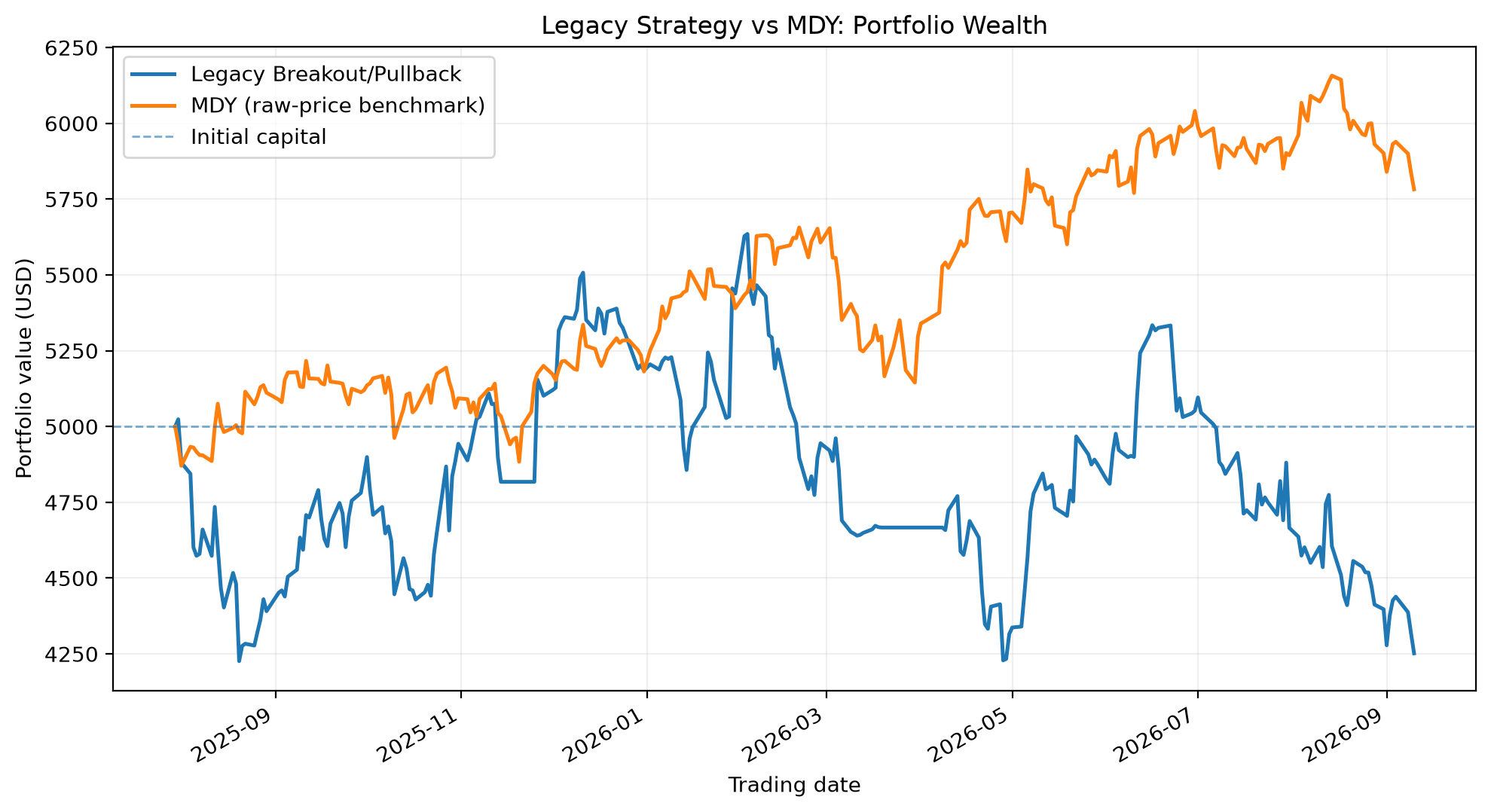
Common-period Legacy strategy wealth versus the MDY raw-price benchmark

Figure 1. Portfolio wealth on the common calendar. Strategy execution includes modelled costs; the normalised MDY comparator excludes distributions and transaction costs.

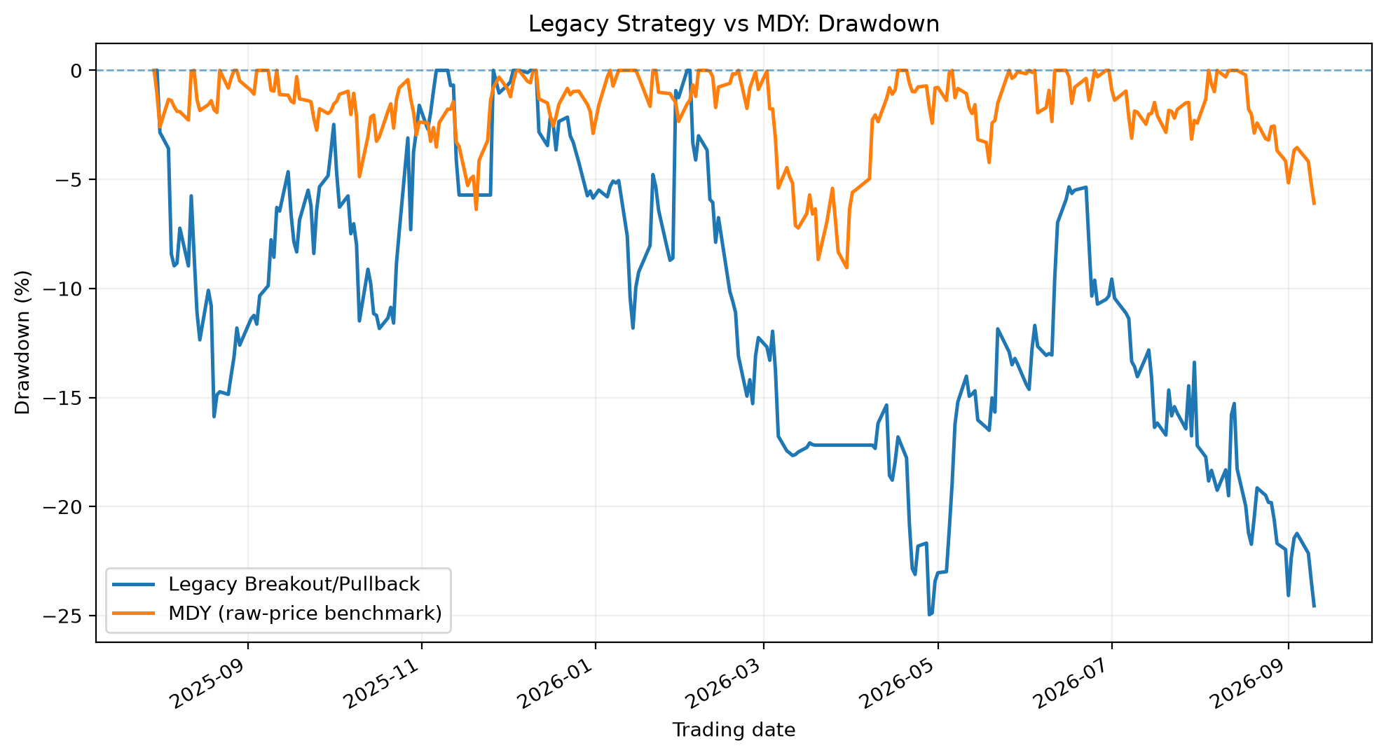
Drawdowns for the Legacy strategy and MDY

Figure 2. Percentage drawdown from each wealth series’ running peak.

5.3 Results by setup

Statistic	Breakout	Pullback
Closed trades	35	25
Winners	15	7
Win rate	42.86%	28.00%
Mean net return per trade	+0.34%	−2.49%
Median net return per trade	−5.00%	−5.47%
Total net realised P&L (USD)	+504.13	−1,252.23
Profit factor	1.2005	0.4632
Mean counted holding bars	7.14	8.12
Trailing activated	40.0%	28.0%

Table 2. The breakout and pullback labels represent transactions from the same capital-constrained portfolio, not independently funded strategy arms. The notebook’s bars_held counter increments only when a position survives the session’s stop check; therefore, a position stopped out on its entry session records zero counted bars. This is an engine-specific holding-bar measure, not elapsed calendar days.

Breakout returns are positive on average but negative at the median. CGNX, VIAV and ROIV contribute approximately USD 1,193.90, accounting for 39.55% of the breakout group’s gross positive P&L. Subtracting these gains arithmetically from the breakout aggregate would leave −USD 689.77, but this calculation is not a counterfactual portfolio backtest: removing transactions would change cash availability, subsequent entries and the portfolio’s opportunity set. Pullbacks contribute the larger net loss, approximately USD 1,252.23.

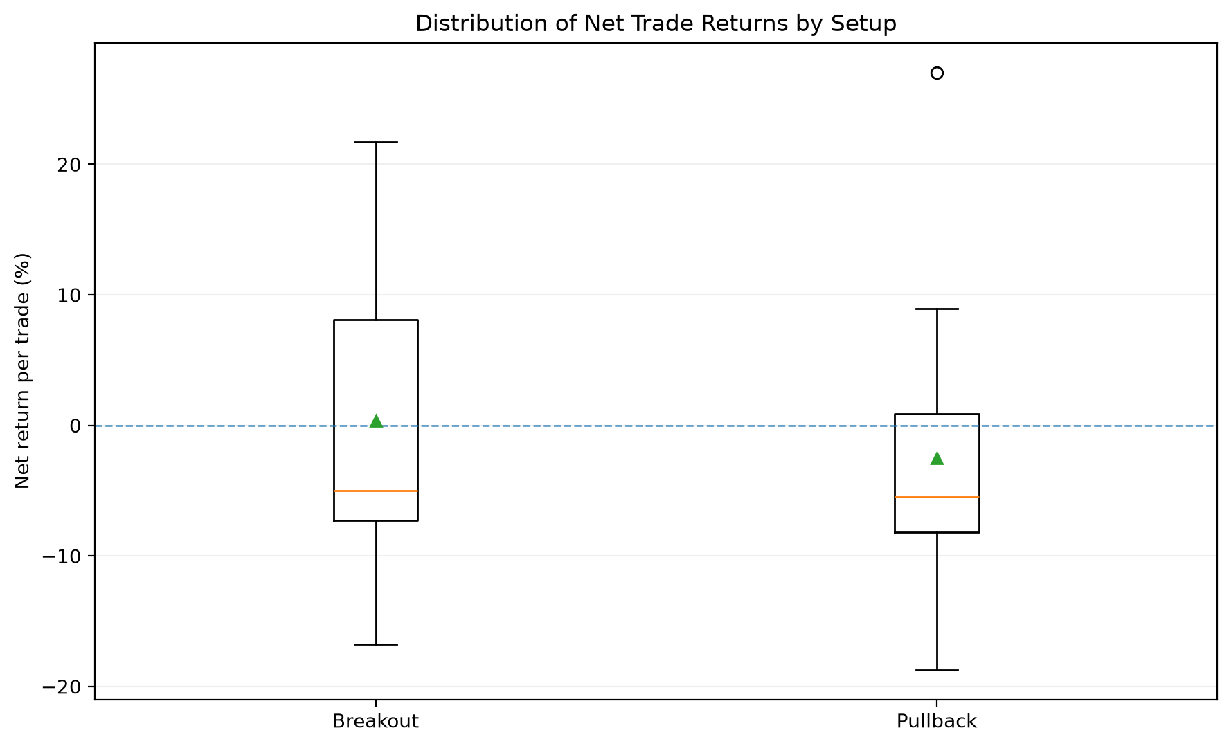
Net trade return boxplots for breakouts and pullbacks

Figure 3. Realised net returns by setup. The central horizontal line is the median and the triangular marker is the mean.

5.4 Temporal performance and gap risk

The active portfolio gains 3.69% during the partial July–December 2025 interval and loses 17.99% during January–10 September 2026; compounding these periods reconciles to approximately −14.96% overall. Neither partial calendar year is an independently funded annual strategy test.

The seven initial gap-stop exits together realise USD 1,350.97 in losses. Their average loss is 1.63 times initial planned price risk; four exceed 1.25 times that allowance. The 29 ordinary initial-stop exits average 1.03 times planned risk, partly because realised P&L includes slippage and commissions omitted from the initial price-distance constraint. Three examples are DY (USD 108.61 planned; USD 276.19 realised), VICR (USD 113.82 planned; USD 266.54 realised) and HIMS (USD 122.03 planned; USD 256.28 realised). A USD 125 nominal risk limit is not a guaranteed maximum loss.

One profitable ARWR breakout coincides with a 23.34% closing-price increase on 26 November 2025 and exits subsequently through trailing management, generating USD 278.02 net P&L. Corporate reporting and other company announcements provide relevant context for the unusual session, but the research does not claim a verified causal explanation from these prices alone. The observations are retained rather than classified as erroneous solely because the movement is large.

6. Reconciliation with the earlier historical result

The prior historical baseline reports 65 trades, −47.0962% return and USD 2,645.19 ending equity. This notebook’s new, separately funded 2025–2026 portfolio produces 60 trades, −14.9622% return and USD 4,251.89 ending equity. The data snapshot and contemporary constituent list are different; no parameter has been modified to force equality.

Two transactions documented in the author’s archived research notes match the new portfolio closely: HIMS (entry 31 July 2025; exit 5 August 2025; approximately −16.79%) and TTMI (entry 5 August 2025; exit 15 August 2025; approximately −8.17%). Their published entry/exit prices agree with the notebook to reported two-decimal precision. Agreement for two examples is not evidence of equality for all transactions. Different membership, historical observations and rank ordering remain possible explanations for portfolio-level divergence, but the precise contribution of each has not been established.

7. Limitations and conclusion

This analysis has several material limitations. Present-day index membership projected backwards is not survivorship-bias-free. Using Yahoo’s Close series with auto_adjust=False excludes the additional dividend adjustment but does not guarantee complete corporate-action consistency or point-in-time prices; basic OHLC consistency checks cannot establish those properties. Downloaded data and Wikipedia membership may change between notebook executions. The daily-bar execution model cannot observe the true intraday order of highs and lows, and fixed transaction costs omit variable spreads, market impact and broker-specific fill uncertainty. Opening gaps can cause realised losses far beyond intended stop distances. The two-position portfolio is sensitive to rankings, score ties, and transaction sequencing. The MDY comparator is a raw-price, dividend-excluding index without its own execution costs, not an exact total-return investable counterpart.

This work is a retrospective descriptive reconstruction, not a pristine holdout study or a statistical multiple-testing correction. It provides no estimate of prospective profitability. The principal finding is narrow: under the documented rules, capital restrictions and fresh-data snapshot, the Legacy strategy loses money in both historical windows and underperforms MDY during the common period. Breakout gains depend on relatively few successes, while pullbacks and price gaps produce substantial risk. Future work should use point-in-time index membership, split-consistent prices, better transaction-cost modelling and pre-specified prospective tests.

References

Brock, W., Lakonishok, J., & LeBaron, B. (1992). Simple technical trading rules and the stochastic properties of stock returns. The Journal of Finance, 47(5), 1731–1764. https://doi.org/10.1111/j.1540-6261.1992.tb04681.x
Lo, A. W., Mamaysky, H., & Wang, J. (2000). Foundations of technical analysis: Computational algorithms, statistical inference, and empirical implementation. The Journal of Finance, 55(4), 1705–1765. https://doi.org/10.1111/0022-1082.00265
Sullivan, R., Timmermann, A., & White, H. (1999). Data-snooping, technical trading rule performance, and the bootstrap. The Journal of Finance, 54(5), 1647–1691. https://doi.org/10.1111/0022-1082.00163
White, H. (2000). A reality check for data snooping. Econometrica, 68(5), 1097–1126. https://doi.org/10.1111/1468-0262.00152
Zhu, Y., & Zhou, G. (2009). Technical analysis: An asset allocation perspective on the use of moving averages. Journal of Financial Economics, 92(3), 519–544. https://doi.org/10.1016/j.jfineco.2008.07.002

Reproducibility materials

Download the executed Jupyter notebook and pinned dependencies. In the download directory, execute python -m pip install -r requirements.txt and start python -m jupyter lab. Run notebook cells sequentially with a working internet connection. The notebook retrieves its own stock universe and market prices, computes signals, simulates positions and regenerates the research figures. It connects to no brokerage service and transmits no trading orders.

Reproducibility note: Numerical results correspond to an October 2026 data retrieval. They may differ when historical market data or the contemporary constituent universe changes. The accompanying notebook provides the computational implementation and data-integrity checks.