Trading strategies explained · Cenk Ufuk Yildiran · 28 October 2026
When a stock falls sharply, one person sees danger and another sees a bargain. Both might be right. But what if the stock has been rising for months and has simply had a bad week? Could that short setback offer a buying opportunity?
This is the question behind Reversal5, a rule-based trading strategy tested using U.S. mid-cap share prices. Instead of buying the strongest recent performers, the strategy looks for stocks that have fallen unusually hard over the last five trading sessions, even though their longer-term trend is still positive. It buys only if several other conditions are satisfied, then sells quickly.
The full historical simulation made money, but the later results were less impressive, one calendar year was negative, and a simple mid-cap market benchmark did better during the directly comparable period. The result is a lesson about how to test a promising idea—not a reason to rush into buying falling stocks.
This article is a plain-English companion to Post 5: the technical Reversal5 replication. It follows the same approach as Post 2’s guide to breakout and pullback trading and Post 4’s guide to momentum. You do not need to understand Python, statistics or finance formulas.
1. What does “short-term reversal” mean?
Picture a company whose shares have slowly risen from $40 to $60. Then, over five trading days, the price falls to $55. One possible explanation is that some investors have sold too aggressively, creating a temporary price decline. If buyers return, the stock may recover. That possible bounce is called a short-term reversal.
But falling prices can also signal genuinely bad news. A stock is not automatically cheap simply because it fell yesterday, and a rebound is never guaranteed. The strategy therefore looks for a specific combination of short-term weakness and longer-term strength.
A bad week inside a longer upward trend
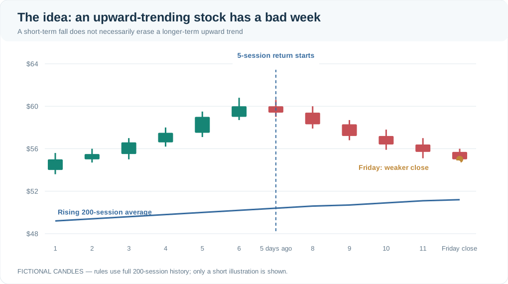
Figure 1. A fictional stock suffers a five-session decline while remaining above its rising longer-term average. A candle’s thick body connects its opening and closing prices; the thin vertical line shows the day’s high and low. Green means the close exceeded the open, while red means it finished below the open. Only a few candles are illustrated; the real moving-average calculation uses 200 sessions.
The blue line is a simplified picture of the stock’s 200-session moving average—the average of roughly ten months of daily closing prices. Reversal5 wants the price above that average and the average itself to be rising. So it is not designed to buy every stock in free fall.
2. How does the system decide which falling stocks to consider?
Once a week, on the last trading session shown by the MDY benchmark (normally Friday), the program checks the stocks in its research list. It uses five trading sessions of price history, not necessarily five calendar days.
Five conditions help narrow the list:
- A genuinely weak five sessions: the share’s closing price must be lower than it was five sessions earlier.
- An established upward trend: the closing price must be above a rising 200-session average.
- A practical share price: at least $10 per share.
- Enough trading activity: at least $5 million of average daily traded value over the past 20 sessions. That is money traded, not the company’s market value.
- Volatility not too extreme: a recent trading-range measure, called average true range, cannot exceed 10% of the share price.
These filters are checked using the information available by the end of the weekly signal session. Unlike the earlier breakout and momentum studies, Reversal5 does not require MDY itself to be in a positive moving-average regime. The trend check applies to the individual share.
“Worse than the market” matters more than “down the most”
Suppose Stock A fell 8%, Stock B fell 4%, and the mid-cap market benchmark MDY fell 2% over the same five sessions. Stock A lagged MDY by 6 percentage points, while Stock B lagged it by 2 percentage points.
That difference is the strategy’s relative reversal score: stock’s five-session return minus MDY’s five-session return. The program ranks eligible stocks from the most negative score upward, breaking ties using the stock’s own return and then its symbol.
It retains roughly the bottom 10% of eligible stocks, not 10% of every stock in the research list. If 50 shares qualify after all the screens, that would mean the five most negative relative performers. A candidate is not yet a trade: the portfolio may have no free cash or spare position slot.
In the executed historical research there were 1,810 weekly ranked candidates across 216 weeks with candidates, but only 368 trades were ultimately opened and closed in the main full-period portfolio.
3. When does it buy? Not at the price used to choose the stock
A common mistake in testing a trading rule is to discover a signal at the end of Friday, then pretend you could have bought the same stock at Friday’s already-known closing price.
Reversal5 does not do that. Its signal is calculated after the weekly session closes, and a possible purchase happens at the next available market session’s opening price, provided the portfolio has room. That opening price may be higher or lower than Friday’s close.
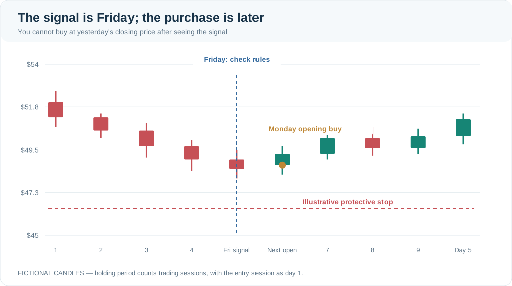
Figure 2. Illustrative weekly signal and next-session purchase. The system ranks at the weekly close but buys no earlier than the next session’s open. The five-session maximum holding period counts the entry session as the first session. This diagram is not a transaction from the historical trade ledger.
How much does it invest?
The simulated account starts with $5,000. It can hold at most two stocks simultaneously and has a $2,500 maximum investment per stock. The share quantity is also restricted so that the planned initial price loss is at most $125 per position, subject to having enough cash.
The model includes $1 for each buy or sell order and an adverse price allowance of 0.05% on both entry and exit. These are simplified assumptions about trading costs, not a guarantee that a real order would get the same fill.
In other words, the strategy does not pour the entire $5,000 account into whichever share has had the worst week.
4. How does it get out? Three exit rules
The word reversal may make it sound as though the strategy waits for a complete recovery. It does not. Reversal5 has a deliberately short clock and predefined exit rules.
Initial stop-loss: on entry, a protective sell level is set below the purchase price. Its distance depends on the stock’s recent trading range, but is limited to 4%–8% of the entry price. A $50 purchase with a 6% initial stop would have a planned exit level near $47.
Trailing stop: if an observed high reaches 7.5% above the executed buy price, a trailing stop becomes active at 5% below the highest observed price. For a fictional $50 purchase, the activation level is $53.75. If a session reaches $54.40, the trailing stop would be approximately $51.68 (5% below $54.40). It can subsequently rise as new highs occur but does not move down.
Time limit: if no stop is triggered, the position is closed at the fifth processed trading session, counting the buy session as day one. The model does not wait indefinitely for an anticipated rebound.
How a winning reversal could end
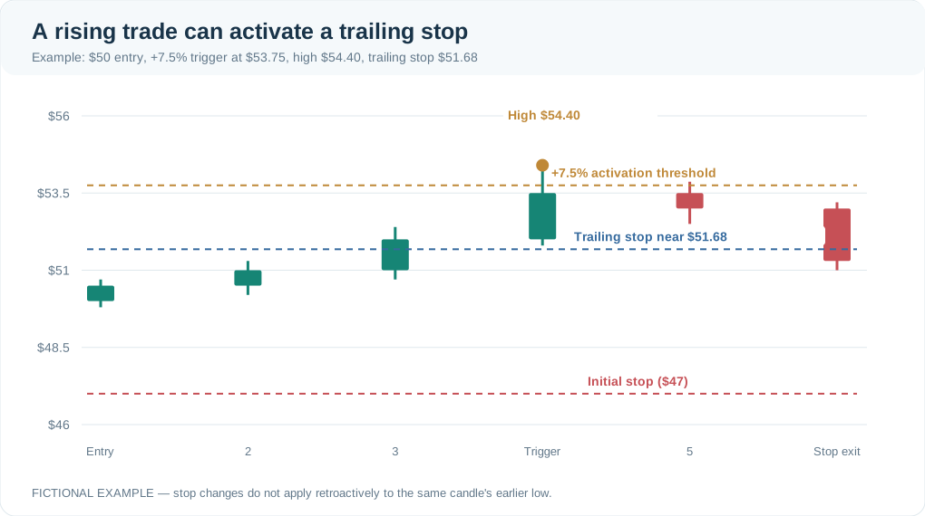
Figure 3. A fictional $50 position climbs enough to activate the 7.5% trigger, then the trailing stop follows 5% below the best observed high. In the actual daily-bar model, stop checks use a conservative order: an updated stop is not applied retroactively to a low that may have occurred earlier in the same session.
Notice the difference between the 7.5% activation threshold and the 5% trailing distance. They are not two profit targets. One decides when the trailing mechanism turns on; the other determines how far below the observed high the stop sits.
The research also tested an earlier 10% activation rule. The final 7.5% choice was selected after historical comparisons; it should not be mistaken for a rule selected blindly before seeing all the data.
5. Why a stop-loss might not stop the loss you expected
Suppose you enter a stock at $50 and place a stop at $47. Bad news breaks after the market closes, and the next session begins at $44.50. There may be no opportunity to sell at $47: the opening price has already jumped below the planned level.
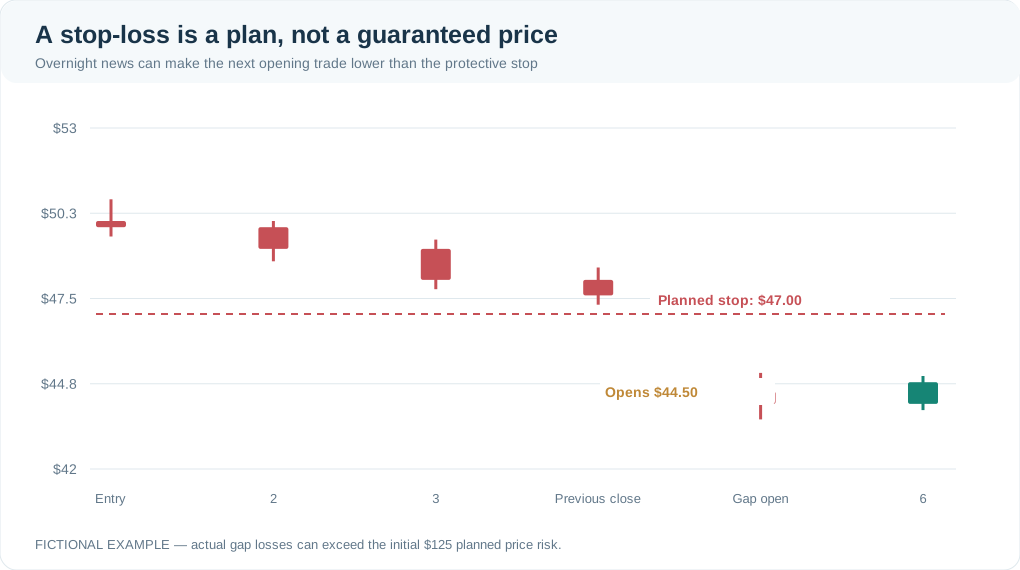
Figure 4. Illustrative overnight gap. A planned $47 exit does not guarantee execution at $47. The model checks for gap-through-stop exits at the next opening price. Actual losses can exceed the initial $125 planned price risk, even when the trade was sized carefully.
This is important because a backtest that simply assumes every stop executes perfectly can make a risky strategy look much safer than it is.
6. What happened to the $5,000 in the historical tests?
Now for the real backtest evidence. The price dataset covers 13 September 2021 to 10 September 2026, allowing the moving averages time to form. The first ranked weekly candidates appear only in late July 2022, after the required history has accumulated.
The main, independently implemented Reversal5 simulation closed 368 trades. Of those, 51.63% finished profitably. The $5,000 starting account grew to $8,526.81, a 70.54% cumulative gain, equivalent to about 11.29% annualised growth over the simulated calendar. The worst fall from a previous portfolio high was 18.11%, and the profit factor was 1.2543—approximately $1.25 in total net winning-trade gains for each $1 in total net losing-trade losses.
Did the choice of trailing-stop trigger matter?
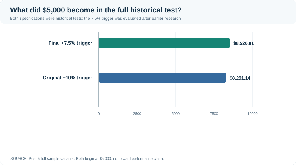
Figure 5. Actual full historical simulation outcomes, both starting at $5,000. The final 7.5% trigger ended at $8,526.81 across 368 trades. The original 10% trigger ended at $8,291.14 across 366 trades. These are historical variants; the difference is not evidence that 7.5% is universally optimal.
The updated trigger produced a somewhat better result in the historical data. But the key word is historical: choosing a parameter after examining past outcomes is different from successfully predicting an unseen future.
Was performance as good in every period?
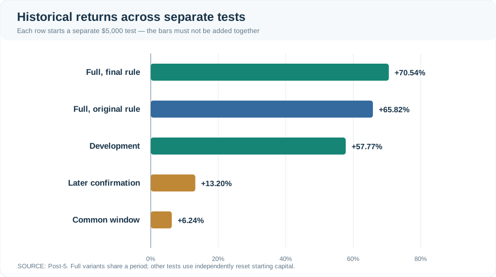
Figure 6. Actual Reversal5 historical results. The full final simulation returned +70.54% (368 trades); the original full-rule variant +65.82% (366); development +57.77% (220); later confirmation +13.20% (148); and the harmonised common period +6.24% (102). Each separately reported test uses its own fresh $5,000 account, so these percentage gains must not be added together.
The later confirmation period was weaker than the development period. It also was not a pristine, untouched out-of-sample test, because earlier research decisions had already involved inspecting later historical data. This limits what we can conclude about genuine predictive power.
7. Did Reversal5 actually beat just holding the mid-cap market?
This is where the answer becomes more cautious.
To make a comparable historical-window assessment, take 30 July 2025 through 10 September 2026. Over those dates, the independently funded Reversal5 portfolio returned +6.24%, turning $5,000 into $5,312.02.
The raw closing price of MDY, an ETF representing the U.S. mid-cap market, increased 15.65% over the same dates. A hypothetical $5,000 measured using that raw price change becomes about $5,782.35.
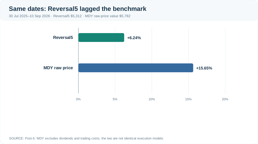
Figure 7. Same historical dates: Reversal5 +6.24%, MDY raw price +15.65%. That is approximately 9.41 percentage points of underperformance for Reversal5. The MDY line excludes dividends and trading costs, while the strategy simulation includes its modelled costs, so this is an informative benchmark comparison rather than two identical executable accounts.
A positive return is not the same thing as a successful strategy. If taking active trading risk produces less growth than a simpler benchmark over the same period, that opportunity cost matters.
8. Some years looked good; one looked poor
The researchers also ran a separate experiment in which the $5,000 account was reset at the beginning of each calendar-year test. The returns varied considerably:
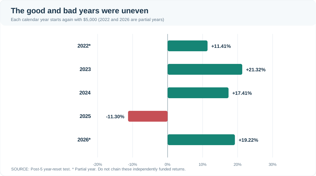
Figure 8. Independent annual reset tests: 2022 +11.41% (partial), 2023 +21.32%, 2024 +17.41%, 2025 −11.30%, and 2026 +19.22% through 10 September. The negative 2025 is not a minor graphical detail: it shows a year in which the strategy lost money. Because every year starts with a new $5,000, do not multiply these bars together as though they were consecutive returns from one account.
The 2025 result is a reminder that a profitable full-history backtest can hide difficult shorter intervals. The separately funded later confirmation test also experienced a maximum peak-to-trough fall of approximately 20.42%.
9. What ended the trades: recovery, a stop, or the clock?
Most positions did not actually reach a dramatic trailing-stop exit. The main 368-trade historical ledger records:
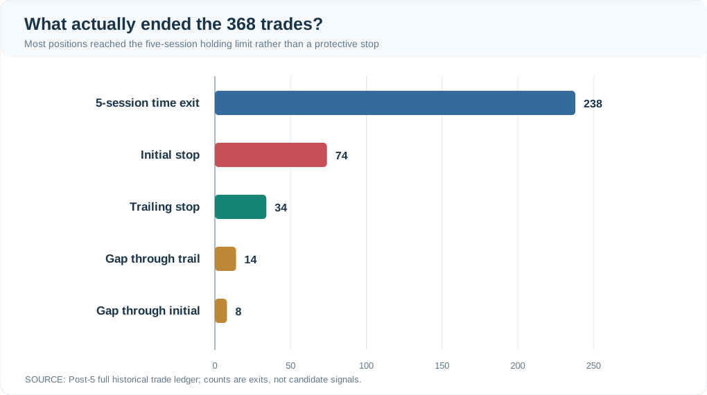
Figure 9. Actual reasons for closing 368 historical trades: 238 hit the five-session time limit; 74 hit an ordinary initial stop; 34 exited via a regular trailing stop; 14 gapped through a trailing stop; 8 gapped through an initial stop. The counts sum to 368. Only 23.91% of trades ever activated the trailing rule.
This reinforces the strategy’s defining feature: it is a short-lived bet on a possible rebound, with limited patience. The most common outcome is not a big recovery that locks in profits; it is simply reaching the scheduled end of a five-session holding window.
10. What does this backtest prove—and what doesn’t it?
Three ideas are worth separating.
The rules are reproducible. Post 5 independently rebuilt the simulator in Python and reconciled five sets of trade counts, total returns and profit factors against the original working-paper reference to four decimal places. That is a useful check of computation and documentation.
The historical results are mixed. The full-period portfolio was profitable, but the subsequent historical confirmation was weaker, 2025 was negative in the annual reset experiment, and the strategy underperformed MDY in the common comparison window.
Neither of these facts establishes future success. The 399-stock research list is a reconstruction of the original paper’s selected universe, not a complete record of all firms that historically entered or left the S&P MidCap 400. Missing delisted companies can produce survivorship bias. Vendor historical prices can change; simplified daily candles cannot reveal the actual intraday order of every price movement; and small slippage assumptions do not capture all real trading costs. The study is retrospective, not prospective live validation.
The bottom line: buying a dip is easy to explain, but hard to prove
Reversal5 asks a sensible question: could a temporarily weak stock recover when its longer trend is still healthy? It turns that idea into exact rules for eligibility, ranking, next-session entries, position sizing, protective stops and a short holding period.
The complete backtest produced a positive historical return. Yet its later results and benchmark comparison put an important limit on the story. A strategy can make money in a backtest without demonstrating that it is a better or more dependable choice than the market.
For the equations, research design, full comparison tables, methodological limitations, downloadable executed notebook and data-provenance files, read Post 5: Reversal5 — Reconstructing Weekly Short-Horizon Reversal in Python.
Educational research commentary only. This is not personalised financial advice or a recommendation to buy or sell securities. Figures 1–4 are fictional candlestick illustrations; Figures 5–9 are charts of archived historical research results.