Reversal5: Reconstructing Weekly Short-Horizon Reversal in Python

Computational finance · Cenk Ufuk Yildiran · 28 October 2026

Abstract

This article independently reconstructs Reversal5, the weekly, long-only short-horizon contrarian trading policy described in From Breakouts and Momentum to Short-Term Reversal. It uses the same fixed, 399-stock reconstructed original-paper universe as the Momentum52 replication, not a new Wikipedia index snapshot, while independently retrieving daily stock and benchmark prices from Yahoo Finance. A transparent Python/Jupyter implementation imposes the original eligibility, relative-return ranking, capital allocation, execution timing, trading costs, stops and five-session holding rule.

Executed historical replication: the final +7.5% trailing-activation specification generated 368 closed trades, +70.5363% cumulative portfolio return, 11.2874% annualised growth, −18.1064% maximum drawdown and 1.2543 profit factor; USD 5,000 ended at USD 8,526.81. The independently funded development, previously inspected confirmation and common-comparison windows respectively produced +57.7686% (220 trades), +13.1998% (148 trades) and +6.2405% (102 trades). The separately reconstructed original +10% trailing-trigger specification returned +65.8228% (366 trades). All five trade-count, return and profit-factor summaries agree with the earlier paper to four decimal places. However, in the common window, the raw-price MDY benchmark gained 15.6469%, exceeding Reversal5. These are retrospective reproductions, not new prospective validation or evidence of a broadly persistent investment edge.

Research downloads: executed Jupyter notebook · Python requirements · frozen 399-stock CSV · stock-universe provenance · paper reconciliation CSV · results summary JSON · download coverage audit.

1. Literature review and research hypothesis

1.1 Why study recent losers?

Very-short-horizon reversal concerns the possibility that securities with unusually poor recent returns subsequently rebound. Lehmann (1990) documents a tendency for weekly winners and losers to reverse during the subsequent week, with careful discussion of measurement and transaction costs. Jegadeesh (1990) identifies return predictability and negative serial correlation at shorter lags in stock returns. These findings motivate the five-session formation window; neither establishes that buying two weekly mid-cap losers under the particular constraints used here should outperform.

1.2 Mechanisms and implementation frictions

Lo and MacKinlay (1990) show that contrarian returns may reflect cross-autocovariances and lead–lag effects rather than simple individual-stock overreaction. Campbell, Grossman and Wang (1993) relate trading volume to serial correlation and temporary price pressure. Avramov, Chordia and Goyal (2006) examine liquidity and stock-return autocorrelations. Nagel (2012) interprets short-term reversal returns as a proxy for liquidity-provision compensation, particularly when market liquidity is strained. Da, Liu and Schaumburg (2014) distinguish price movements related to fundamental news from nonfundamental shocks.

These are possible economic interpretations, not causal findings of this notebook. A two-position strategy with daily historical bars cannot separately identify inventory effects, bid–ask bounce, stale pricing, information shocks or investor behaviour. More broadly, transaction costs and repeated strategy search may substantially weaken apparent backtest opportunities.

1.3 Reversal within a longer-term positive trend

Reversal5 combines short-horizon weakness with a positive and rising 200-session moving average. The purpose is to test temporary weakness within a longer-term stock uptrend, rather than mechanically buying any recent loser. Research on moving-average rules and cross-sectional technical analysis (for example, Zhu and Zhou, 2009; Han, Yang and Zhou, 2013) provides context, but does not validate these exact thresholds. The implementation is a historical project-specific design retained unchanged in this replication.

Research question: Can a fixed weekly bottom-decile relative-loser rule, after executable capital constraints and simplified costs, reproduce the original paper’s historical portfolio outcomes without hindsight parameter changes?

2. Frozen universe and independently sourced prices

The stock universe is the fixed 399-ticker CSV used in Post 3, with its membership-reconstruction provenance and SHA-256 fingerprint. The list was inferred from the original-paper/Post-1 reconciliation (393 overlapping names, six original-only names, seven Post-1-only names). It is not a byte-identical archived copy of the original trading-system constituent file, and it is not point-in-time S&P MidCap 400 membership. Former index constituents and delisted losers can therefore be absent: survivorship and delisting biases remain.

The notebook fetched 399 stock histories plus MDY, the SPDR S&P MidCap 400 ETF Trust, through the Yahoo Finance interface in Python, over 13 September 2021–10 September 2026 inclusive. The MDY reference calendar has 1,254 sessions. The download settings were daily frequency, no automatic dividend adjustment, no automatic repair and no corporate-action tables: auto_adjust=False, repair=False, actions=False. Yahoo’s Close series may already reflect stock-split adjustments, so these are not necessarily entirely unadjusted historical prices. Download-vintage changes remain possible.

All 399 named stock histories were retrieved; 398 passed the minimum-history condition, while SOLS had only 224 available observations and could not enter signal generation. No ticker was silently substituted. The downloaded records and vendor-software versions were fingerprinted; see the download audit and the notebook-generated local price manifest. Provider price caches are intentionally not included in the publication package.

The research window begins in September 2021 to provide sufficient historical prices, but the weekly signals begin only after rolling-indicator warm-up; the first ranked candidate signal occurred on 29 July 2022, for a next-session entry. This distinction matters when interpreting whole-calendar annualisation.

3. Formal mathematical specification

Let $O_{i,t},H_{i,t},L_{i,t},C_{i,t},V_{i,t}$ denote the stock’s daily open, high, low, close and volume. Subscript $M$ denotes MDY. All signal information is available on the signal date, not taken from the future execution bar.

3.1 Five-session stock and benchmark returns

r_{i,t}^{(5)} = \frac{C_{i,t}}{C_{i,t-5}}-1,\qquad r_{M,t}^{(5)} = \frac{C_{M,t}}{C_{M,t-5}}-1.

The ranking score is the difference between stock and benchmark returns:

RR_{i,t}^{(5)} = r_{i,t}^{(5)}-r_{M,t}^{(5)}.

A more negative value denotes more pronounced five-session underperformance of MDY. This return-difference construction is not a beta-neutral hedge: Reversal5 buys individual stocks and never shorts MDY.

3.2 Trend, dollar-volume liquidity and volatility

The 200-session simple moving average and its 20-session slope are

SMA_{i,t}^{(200)}=\frac{1}{200}\sum_{j=0}^{199}C_{i,t-j}, \qquad \Delta_{20}SMA_{i,t}^{(200)}=SMA_{i,t}^{(200)}-SMA_{i,t-20}^{(200)}.

The average daily traded dollar value is the mean of daily price–volume products,

ADV_{i,t}^{(20)}=\frac{1}{20}\sum_{j=0}^{19}C_{i,t-j}V_{i,t-j}.

True range and 14-session average true range are

TR_{i,t}=\max\!\left\{ H_{i,t}-L_{i,t},\, |H_{i,t}-C_{i,t-1}|,\, |L_{i,t}-C_{i,t-1}| \right\}, \quad ATR_{i,t}^{(14)}=\frac{1}{14}\sum_{j=0}^{13}TR_{i,t-j}.

This ATR is an arithmetic average of true ranges, not Wilder’s recursively smoothed ATR.

3.3 Eligible weekly signals and bottom-decile selection

The signal date is the last available MDY trading session of each ISO calendar week, including holiday-shortened weeks. Each stock must have an actual observed price bar on that session. Eligibility requires all of:

C_{i,t}\ge10,\quad ADV_{i,t}^{(20)}\ge5{,}000{,}000,\quad C_{i,t}>SMA_{i,t}^{(200)},\quad \Delta_{20}SMA_{i,t}^{(200)}>0,

r_{i,t}^{(5)}<0,\qquad \frac{ATR_{i,t}^{(14)}}{C_{i,t}}\le0.10.

Unlike Legacy Breakout/Pullback and Momentum52, Reversal5 does not require a positive MDY SMA50/SMA200 market-regime gate. The long-term trend filter applies to the individual stock.

Among $N_t$ qualifying stocks, rank in ascending order of $RR_{i,t}^{(5)}$ ; break exact ties using the raw stock five-session return, then symbol. Keep

K_t=\max\!\left(1,\left\lceil0.10N_t\right\rceil\right).

Thus, the bottom decile is formed after eligibility screening, not from the entire 399-stock list. The executed calendar contained 216 weeks with candidates and 1,810 retained bottom-decile proposals. These are eligible ranked proposals, not 1,810 executed trades.

3.4 Next-session execution, sizing and protective stops

Signals formed at the weekly closing price can be traded only at the next MDY-session open, with adverse entry slippage of five basis points:

P_i^{entry}=O_{i,t+1}(1+0.0005).

The signal-date ATR fixes the trade’s initial stop percentage:

s_{i,t}=\min\!\left(0.08,\max\!\left[0.04,\, \frac{1.5ATR_{i,t}^{(14)}}{C_{i,t}}\right]\right).

The initial stop is $P_i^{stop}=P_i^{entry}(1-s_{i,t})$ . The USD 5,000 portfolio permits two simultaneous long positions, maximum USD 2,500 capital per stock, at most USD 125 planned initial price risk per trade, and no more than two new orders in a session. The whole-share quantity is

q_i=\min\!\left\{ \left\lfloor\frac{125}{P_i^{entry}s_{i,t}}\right\rfloor,\, \left\lfloor\frac{2500}{P_i^{entry}}\right\rfloor,\, \left\lfloor\frac{Cash_{available}-1}{P_i^{entry}}\right\rfloor \right\}.

The final Reversal5 variant activates a 5% trailing stop after a 7.5% favourable high-price move relative to executed entry. The trailing anchor is the highest relevant observed price since activation, while the stop cannot move down:

A_{i,t}=\max(A_{i,t-1},H_{i,t}),\qquad P_{i,t}^{trail}=\max(P_{i,t-1}^{stop},0.95A_{i,t}).

The simulator processes gap-through-stop exits at the opening price first, then any newly financeable entries, and applies the previous effective stop before updating the trail within a daily bar. A newly raised stop is not applied retroactively to an earlier low on the same day. Surviving positions exit at the fifth processed trading session, counting the entry session as one. Sales incur five basis points adverse slippage and USD 1 commission per order. Overnight gaps can create realised losses larger than the USD 125 intended price-risk amount.

3.5 Portfolio accounting and evaluation statistics

Marked-to-market equity and running drawdown are

E_t=Cash_t+\sum_{i\in Holdings_t}q_iC_{i,t},\qquad DD_t=\frac{E_t}{\max_{s\le t}E_s}-1.

Total return is $E_T/5000-1$ , annualised growth uses elapsed calendar years, and profit factor is total positive realised net trade P&L divided by the absolute value of total negative realised net trade P&L. Development, confirmation, common-period and calendar-year robustness runs each start with a separately funded USD 5,000 account; their gains must not be added together as though they formed one continuous equity curve.

4. Executed replication results

4.1 Primary historical portfolio comparisons

Historical window / policy	Trades	Win rate	Total return	CAGR	Max drawdown	Profit factor	Ending equity
Full calendar, final +7.5%	368	51.63%	+70.5363%	11.2874%	−18.1064%	1.2543	$8,526.81
Development, final +7.5%	220	53.18%	+57.7686%	20.2777%	−14.3269%	1.3710	$7,888.43
Later confirmation, final +7.5%	148	50.00%	+13.1998%	7.8127%	−20.4198%	1.1087	$5,659.99
Common comparison, final +7.5%	102	50.98%	+6.2405%	5.5828%	−17.2726%	1.0774	$5,312.02
Full calendar, original +10%	366	50.00%	+65.8228%	10.6642%	−18.0348%	1.2360	$8,291.14

Table 1. Outputs of the newly executed independent notebook using its frozen member list and cached newly retrieved Yahoo Finance price snapshot. The development window is 28 July 2022–15 January 2025, later confirmation 16 January 2025–10 September 2026, and common comparison 30 July 2025–10 September 2026. The full research calendar is 13 September 2021–10 September 2026, with initial indicator warm-up.

The independent reconciliation records five matches out of five for trade counts, total returns and profit factors to four decimal places against the published working-paper reference. This is a substantial computational-replication result. It does not establish byte-for-byte equality of original OHLCV data, equality of every transaction in an archived private ledger, or independently generated forward evidence. The reconciliation CSV and full summary JSON provide audit-ready numeric comparisons.

4.2 Common-period opportunity cost versus MDY

The independently funded common-period Reversal5 portfolio returned +6.2405%. Over the same dates, MDY’s raw-price close-to-close total change was +15.6469% (dividends excluded). On this comparison, the strategy therefore lagged MDY by approximately 9.41 percentage points. An executable MDY buy-and-hold calculation with next-open execution costs is a different comparator; this figure uses raw MDY closing prices, not the full total-return dividend series.

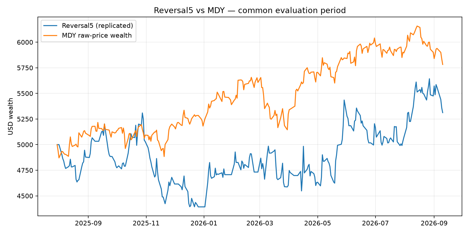
Reversal5 and the MDY raw-price benchmark, independently normalised to USD 5,000 at the common comparison start.

Figure 1. Common-period marked-to-market portfolio equity versus MDY raw-price wealth, 30 July 2025–10 September 2026. Both start at USD 5,000. The MDY line omits distributions.

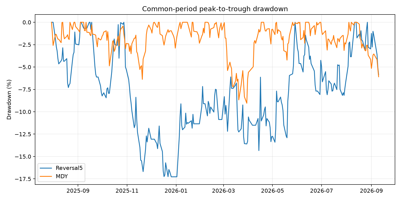
Peak-to-trough percentage drawdowns for Reversal5 and MDY during the common comparison window.

Figure 2. Common-period drawdown paths. Reversal5’s full-historical maximum drawdown is −18.1064%; its separately funded common-period maximum is −17.2726%. These are distinct samples.

4.3 Year-reset robustness and instability

Separately funded calendar year	Trades	Return	Profit factor
2022 (partial)	40	+11.4082%	1.3660
2023	87	+21.3202%	1.4052
2024	91	+17.4072%	1.2541
2025	87	−11.3003%	0.8676
2026 (partial through 10 September)	64	+19.2227%	1.4698

Table 2. Independent USD 5,000 reinitialisation for each calendar year, rather than annual returns sliced from one continuously compounded portfolio. These rows are sensitivity diagnostics and must not be chained.

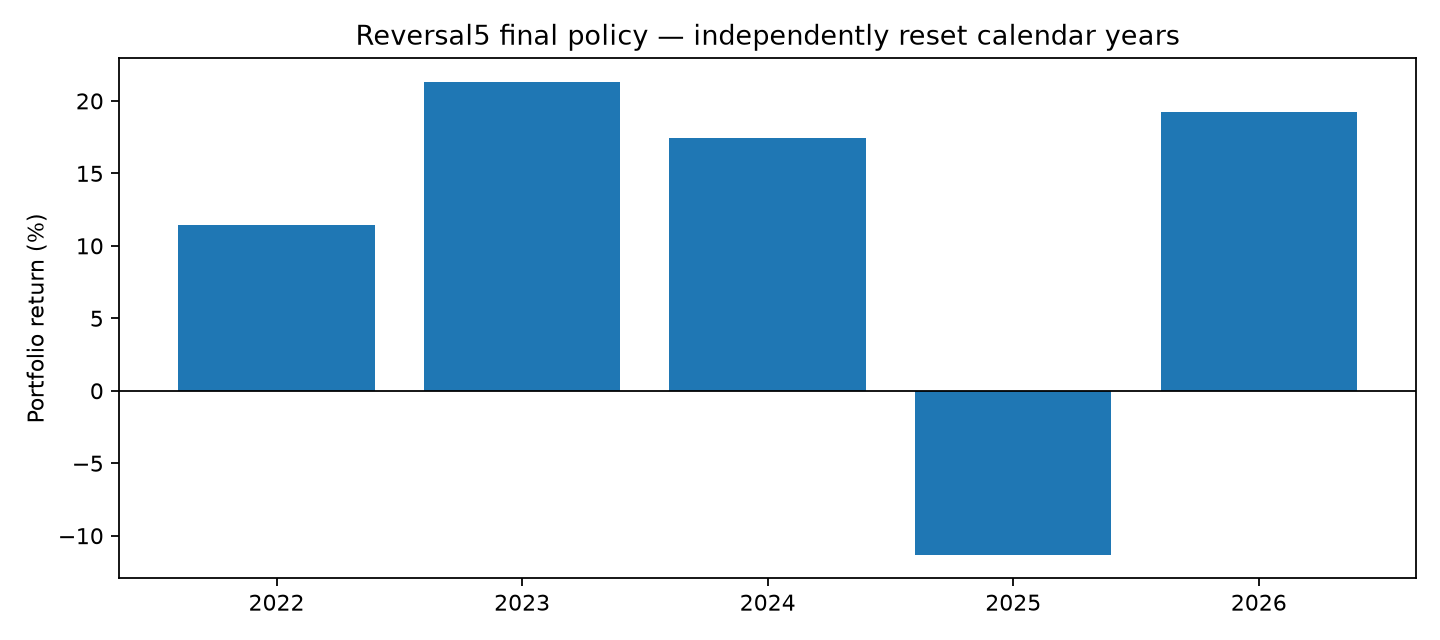
Reversal5 year-reset portfolio returns, showing a negative 2025 amid positive historical years.

Figure 3. The negative 2025 episode demonstrates that positive full-period performance was neither uniform nor assured.

5. Transaction diagnostics and audit trail

The complete historical Reversal5 trade ledger contains 238 five-session time exits, 74 initial-stop exits, 34 standard trailing-stop exits, 14 opening gaps through trailing stops, and 8 opening gaps through initial stops. Only 23.91% of trades registered trailing activation. Time exits therefore form the largest single exit category; the trailing-profit rule is important to some outcomes but does not describe how most trades terminate.

The notebook checks the fixed-universe checksum, formula test cases, benchmark-calendar alignment, weekly candidate rank, position limits, stop ordering, next-session timing, paper-reference tolerance and basic transaction accounting. It saves the ranked signal calendar, independently funded trade and equity ledgers, year-reset diagnostics, stock data-coverage audit and OHLCV hashes in the private research workspace. These facilitate further verification, but do not constitute a completely independent transaction-by-transaction audit against the original archived working-paper database.

The new historical Yahoo snapshot produced numerical agreement with the original paper without parameter changes after observing results. The notebook also reconstructs the original +10% activation setting separately rather than treating the final +7.5% rule as the only strategy ever examined.

6. Evidence classification and research limitations

The strategy lineage is crucial. The original Reversal5 holding-period and trailing-activation choices were evaluated historically; the subsequent +7.5% specification was selected from development-period sensitivity testing after the later period had already been inspected. Accordingly:

Historical reproduction: the original paper’s known numerical results can be regenerated by a separately coded notebook and a frozen stock-list reconstruction.
Development: parameter-selection evidence, including the favourable +7.5% activation in development, is in-sample research.
Later confirmation: 16 January 2025–10 September 2026 results are retrospective confirmation not an untouched out-of-sample selection test.
Harmonised common comparison: 30 July 2025–10 September 2026 compares the strategies over a common historical window, not an independent new experiment.
Genuine forward evidence: would require future frozen signals, later observed outcomes and unchanged rules; that evidence is not generated here.

Principal constraints include survivorship/delisting bias from fixed contemporary membership; vendor revision and corporate-action uncertainty; bid–ask spread, gaps and slippage represented only approximately; daily OHLC bars without intraday price ordering; two-stock concentration; ignored taxes and dividends in the MDY raw-price line; and repeated research decisions over known historical dates. We do not infer an underlying liquidity or behavioural mechanism causally. The paper’s cost-stress results for the original +10% version should not be misrepresented as new stress tests of the final +7.5% version.

Conclusion. Reversal5 is reproducible within the specified research environment, but reproducibility is not the same as a verified forward investment edge. Its positive historical full-period return must be read alongside the weaker later confirmation, negative 2025 year, MDY common-period underperformance and the need for genuine prospective evidence.

7. Reproducibility materials

The downloadable, executed notebook includes its mathematical specification, data-download logic, independent portfolio simulation, figures and saved diagnostic outputs. The frozen ticker list is accompanied by a membership provenance record and requirements file. The paper reconciliation, results summary and download audit allow readers to verify the reported metrics and data coverage. Notebook output text has been scrubbed of local computer paths; this does not change the computed values.

For a reproduction, place the notebook and frozen CSV in the same working directory, install the stated dependencies, and run with Python/Jupyter in a fresh environment with Yahoo Finance access. New Yahoo requests may produce a different data vintage, so exact historical output is not promised unless the original local price snapshot is retained. Data fingerprints can identify disagreement, but cannot themselves recreate market prices.

The notebook neither transmits orders nor connects to a broker. These materials are for historical research, not personalised investment advice.

References

Avramov, D., Chordia, T., & Goyal, A. (2006). Liquidity and autocorrelations in individual stock returns. Journal of Finance, 61(5), 2365–2394.
Brown, S. J., Goetzmann, W. N., Ibbotson, R. G., & Ross, S. A. (1992). Survivorship bias in performance studies. Review of Financial Studies, 5(4), 553–580.
Campbell, J. Y., Grossman, S. J., & Wang, J. (1993). Trading volume and serial correlation in stock returns. Quarterly Journal of Economics, 108(4), 905–939.
Da, Z., Liu, Q., & Schaumburg, E. (2014). A closer look at the short-term return reversal. Management Science, 60(3), 658–674. https://doi.org/10.1287/mnsc.2013.1766
Han, Y., Yang, K., & Zhou, G. (2013). A new anomaly: The cross-sectional profitability of technical analysis. Journal of Financial and Quantitative Analysis, 48(5), 1433–1461.
Jegadeesh, N. (1990). Evidence of predictable behavior of security returns. Journal of Finance, 45(3), 881–898. https://doi.org/10.1111/j.1540-6261.1990.tb05110.x
Lehmann, B. N. (1990). Fads, martingales, and market efficiency. Quarterly Journal of Economics, 105(1), 1–28. https://doi.org/10.2307/2937816
Lo, A. W., & MacKinlay, A. C. (1990). When are contrarian profits due to stock market overreaction? Review of Financial Studies, 3(2), 175–205.
Nagel, S. (2012). Evaporating liquidity. Review of Financial Studies, 25(7), 2005–2039. https://doi.org/10.1093/rfs/hhs066
Yildiran, C. U. (2026). From Breakouts and Momentum to Short-Term Reversal: Sequential Strategy Development and Out-of-Sample Validation in U.S. Mid-Cap Equities. SSRN working paper. https://papers.ssrn.com/sol3/papers.cfm?abstract_id=7636019